From Classroom Algebra to Modern Econometrics: How Equation Subtraction Powers Regression

Most students first encounter the technique in introductory algebra: line up two lines, draw a horizontal rule, and subtract the second equation from the first to erase an unknown variable. The exercise feels purely mechanical, a neat paper-and-pencil trick to solve for x and y before moving on to the next textbook chapter. Outside secondary school classrooms, that exact algebraic reflex serves as the structural backbone for causal inference across tech platforms, macroeconomic forecasting, and observational medicine.
When researchers attempt to measure whether an intervention actually works, whether an interest rate adjustment curbs inflation, an ad algorithm increases conversions, or a new drug lowers blood pressure, the central hurdle is confounding noise. Hidden traits that do not change over time often distort raw correlation. By structuring paired observations and subtracting one from another, data scientists strip away static background variables without ever measuring them directly. As highlighted in a recent Investopedia Report exploring modern hypothesis testing and two-sample t-test variations, isolating genuine differences from random noise remains the cornerstone of empirical investigation. What begins as algebraic cancellation ends as the engine of econometric credibility.
📌 Key Takeaways:
- The Core Mechanism: Subtracting one linear relation from another triggers an algebraic cancellation that purges unobserved, time-invariant confounders.
- The Econometric Engine: Both the difference-in-differences design and the fixed effects estimator rely fundamentally on equation differencing to isolate causal effects.
- The Statistical Trade-off: Differencing removes nuisance variables cleanly, but it burns degrees of freedom and magnifies high-frequency measurement noise.
The Elimination Method That Refuses to Retire
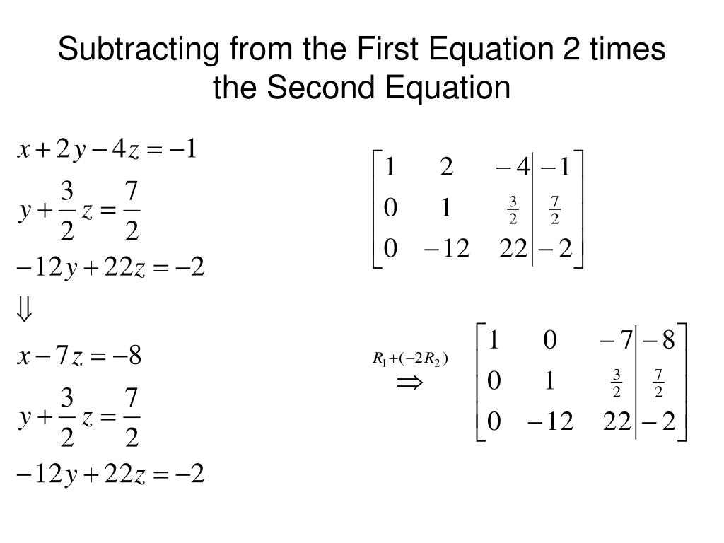
In standard high school algebra, the elimination method handles a basic system of linear equations. If $2x + y = 10$ and $x + y = 6$, subtracting the second line from the first instantly wipes out $y$, leaving $x = 4$. The beauty of the move lies in its simplicity. You do not need to discover what $y$ is doing independently before resolving $x$; you simply delete it from the system through simple arithmetic.
That exact behavior solves one of the most frustrating barriers in modern linear regression. In observational studies, outcome variables are driven by thousands of inputs. Many of these independent variables, such as a company's internal corporate culture, a worker's innate ambition, or an ecosystem's soil composition, cannot be quantified cleanly. When an analyst runs an ordinary least squares model without measuring these attributes, omitted variable bias corrupts the estimates. The solution is rarely better measurement. It is subtraction.
Difference-in-Differences and the Search for Counterfactuals
Consider the classic econometric modeling challenge of assessing a minimum wage hike across state borders. Suppose New Jersey raises its hourly floor, while neighboring Pennsylvania leaves its rate unchanged. Comparing post-policy employment between the two states provides misleading results because New Jersey and Pennsylvania have structurally different economies, living costs, and labor densities.
Economists solve this with difference-in-differences estimation, a method built on two distinct rounds of equation subtraction:
First, analysts take the post-treatment employment equation for New Jersey and subtract its pre-treatment baseline. This removes all permanent, baseline characteristics unique to New Jersey that existed before the law changed. Second, analysts perform the identical subtraction on Pennsylvania's timeline, netting out regional trends that occurred over the same calendar window. Finally, subtracting the second equation from the first leaves behind only the treatment effect. Unobserved state characteristics vanish from the ledger because they entered both time periods with identical values.
Differencing Strategies Across Quantitative Frameworks
The core logic of subtraction reappears across multiple empirical methodologies, ranging from simple group tests to large-scale longitudinal regressions. The mathematical mechanics change, but the strategic outcome remains consistent across disciplines.
| Method | Mathematical Operation | Target of Cancellation | Primary Application |
|---|---|---|---|
| Algebraic Elimination | $Row_1 - Row_2$ in matrix systems | Co-occurring linear variables | Solving deterministic systems |
| Two-Sample T-Test | Subtracting group mean $\bar{X}_2$ from $\bar{X}_1$ | Shared background expectations | Basic hypothesis testing |
| First-Difference Estimator | $Y_{it} - Y_{it-1}$ across panel waves | Unit-specific fixed traits ($\alpha_i$) | Longitudinal panel tracking |
| Difference-in-Differences | $(\Delta Y_{Treatment}) - (\Delta Y_{Control})$ | Common macro shocks and baselines | Public policy evaluation |
How the Fixed Effects Estimator Cleans Longitudinal Data
When tracking panel data across hundreds of firms over several decades, writing individual dummy variables for every single firm devours computing power and inflates parameter counts. Econometricians sidestep this bottleneck using the fixed effects estimator, frequently calculated via the within-transformation.
The mathematical proof relies on taking a baseline equation for firm $i$ at time $t$:
Yit = β Xit + αi + εit
Here, $\alpha_i$ represents unobserved managerial capability, a factor impossible to measure reliably. Next, calculate the time-averaged version of that exact equation for firm $i$ across all recorded years:
Ȳi = β X̄i + αi + ε̄i
Subtracting the second equation from the first produces a transformed model containing only deviations from the mean: $(Y_{it} - \bar{Y}_i) = \beta (X_{it} - \bar{X}_i) + (ε_{it} - \bar{ε}_i)$. The unobserved variable $\alpha_i$ drops out completely. Because its value never drifted over time, subtracting the historical mean equation vaporized it. Ordinary least squares can now estimate $\beta$ without suffering from omitted variable bias.
The Noise Penalty: What Differencing Takes Away
Subtracting linear equations delivers undeniable causal clarity, but it comes at an objective cost. The operation is not free. When analysts subtract one wave of panel observations from another, they discard a massive portion of the dataset's total variance.
Every differencing step extracts a penalty on the model's degrees of freedom. If a researcher works with an experimental panel of 1,200 entities observed over two time periods, first-differencing compresses those 2,400 raw entries into 1,200 change metrics. That halves the effective sample size for temporal variation. If independent variables do not change quickly over time, such as educational attainment or geographical proximity, differencing strips their signal entirely, rendering their effects unidentifiable.
Differencing also compounds high-frequency measurement error. If an outcome variable includes white noise, taking the difference between two noisy readings doubles the variance of the underlying error term while shrinking the signal of slowly evolving real-world changes. Researchers who enthusiastically subtract their way out of omitted variable bias frequently run headfirst into inflated standard errors and fragile statistical significance.
Frequently Asked Questions (FAQ)
Q1: Why is subtraction favored over adding equations in empirical econometrics?
A1: Adding equations bundles parameters together, making individual coefficients harder to distinguish. Subtraction creates an algebraic cancellation that knocks out shared, invariant background factors, leaving only the targeted differential effect.
Q2: How does a simple two-sample t-test relate to regression differencing?
A2: A two-sample t-test evaluates whether the difference between two sample means is statistically distinguishable from zero. A bivariate linear regression with a binary treatment dummy yields the exact same numerical coefficient and p-value, proving that mean subtraction and linear regression differencing are algebraically equivalent.
Q3: When should researchers avoid using equation subtraction?
A3: Differencing performs poorly when independent variables remain stable over time, when measurement error in the baseline period is exceptionally high, or when the parallel trends assumption fails in difference-in-differences designs.
The Enduring Reach of Linear Subtraction
Data science continues to adopt machine learning architectures, automated feature extractors, and high-dimensional neural representations. Yet whenever the objective shifts from basic pattern matching to identifying genuine cause and effect, the industry returns to classical econometrics. The core challenge of empirical work has not changed: reality rarely gives researchers clean counterfactuals, and omitted variables lurk inside every observational registry.
The solution remains strikingly elegant. By lining up two structural states, matching their parallel paths, and subtracting the second equation from the first, researchers peel away layers of hidden bias. Middle school algebra does not just help students solve contrived equations on paper. It provides the analytical scalpel that keeps modern empirical science honest.
